Kapitel 9 Vokalformanten im Deutschen als Fremdsprache

Vowel formants in German as a foreign language

Akustische Messungen der ersten beiden Vokalformanten und Vokaldauer mit Praat, durchgeführt von Studierenden während einer Unterrichtsstunde in einem Einführungsseminar zur computerunterstützten Auswertung von deutschen Sprachkorpora und -datensätzen.

9.1 Programme starten

library(tidyverse)
library(scales)
library(readxl)
library(writexl)
library(phonR)
library(extrafont)

9.2 Daten laden & anpassen

9.2.1 Datensatz 1

vokale <- read_xlsx("data/S03_Vokalformanten_Diagramme.xlsx", 
                    sheet ="A1-4_alle") %>% 
  janitor::clean_names() %>% 
  dplyr::select(-studierende) %>% 
  mutate(geschlecht = "f") %>% 
  dplyr::select(sprecherin, geschlecht, vokal, vowel, 
                f1, f2, dauer, lange, wort, phrase) %>% 
  mutate(l1_l2 = ifelse(sprecherin == "Deutsche", "L1", "L2")) %>% 
  mutate(vokal = str_replace(vokal, "F:", "E:")) # %>% 
  # mutate(vowel = vokal)

vokale %>% rmarkdown::paged_table()

9.2.2 Datensatz 2

vergleich <- read_xlsx("data/S03_Vokalformanten_Diagramme.xlsx", 
                       sheet ="A10_Vgl_L1_L2_tab") %>% 
  janitor::clean_names() %>% 
  mutate(phonem = str_replace(phonem, "EE", "E:")) %>% 
  rename(f1_l1 = f1_in_hz,
         f2_l1 = f2_in_hz,
         dauer_l1 = dauer_in_ms,
         vokal = phonem) %>% 
  dplyr::select(-phonem_ipa_1, -phonem_ipa_2)

vergleich %>% rmarkdown::paged_table()

9.2.3 Datensatz 3

Dieser Datensatz wird aus einzelnen Datensätzen, die Messungen von Studierenden enthalten, zusammengesetzt.

df0 <- read.csv("data/Deutsche_formants.Table.csv", stringsAsFactors = FALSE, fileEncoding = "UTF-8") 
df1a <- read.csv("data/Monika_I_formants.Table.csv", stringsAsFactors = FALSE, fileEncoding = "UTF-8") 
df1b <- read.csv("data/Monika_II_formants.Table.csv", stringsAsFactors = FALSE, fileEncoding = "UTF-8") 
df2 <- read.csv("data/Donna_formants.Table.csv", stringsAsFactors = FALSE, fileEncoding = "UTF-8")
df3 <- read.csv("data/Metka_formants.Table.csv", stringsAsFactors = FALSE, fileEncoding = "UTF-8") 
df4 <- read.csv("data/Jasmina_formants.Table.csv", stringsAsFactors = FALSE, fileEncoding = "UTF-8") 
df5 <- read.csv("data/Teodor_II_formants.Table.csv", stringsAsFactors = FALSE, fileEncoding = "UTF-8") 

df0 <- df0 %>% mutate(speaker = "Deutsche")
df1a <- df1a %>% mutate(speaker = "Monika1")
df1b <- df1b %>% mutate(speaker = "Monika2")
df2 <- df2 %>% mutate(speaker = "Donna")
df3 <- df3 %>% mutate(speaker = "Metka")
df4 <- df4 %>% mutate(speaker = "Jasmina")
df5 <- df5 %>% mutate(speaker = "Teodor")

df <- rbind(df0,df1a,df1b,df2,df3,df4,df5)
df %>% rmarkdown::paged_table()

9.3 IPA syms

Die Listen wurden mit Hilfe der Angaben im Wikipedia-Artikel Phonetic symbols in Unicode, Abschnitt 2.2 Vowels erstellt.

list1 <- levels(factor(vergleich$vowel)) %>% paste(collapse = ",")
list2 <- levels(factor(vokale$vowel)) %>% paste(collapse = ",")
list3 <- levels(factor(df$vowel)) %>% paste(collapse = ",")

ipa_list1 <- c(
a = "\u0061",
AA = "\u0251\u02D0",
E = "\u025B",
ee = "\u0065\u02D0",
EE = "\u025B\u02D0",
I = "\u026A",
ii = "\u0069\u02D0",
O = "\u0254",
oe = "\u00F8\u02D0",
OE = "\u0153",
oo = "\u006F\u02D0",
schwa = "\u0259",
U = "\u028A",
uu = "\u0075\u02D0",
Y = "\u028F",
yy = "\u0079\u02D0"
) # %>% paste(collapse = ",")

ipa_list2 <- c(
a = "\u0061",
AA = "\u0251\u02D0",
E = "\u025B",
ee = "\u0065\u02D0",
EE = "\u025B\u02D0",
I = "\u026A",
ii = "\u0069\u02D0",
O = "\u0254",
oe = "\u00F8\u02D0",
OE = "\u0153",
oo = "\u006F\u02D0",
U = "\u028A",
uu = "\u0075\u02D0",
Y = "\u028F",
yy = "\u0079\u02D0"
) # %>% paste(collapse = ",")

ipa_list3 <- c(
a = "\u0061",
AA = "\u0251\u02D0",
E = "\u025B",
Ea = "\u025B\u0061",
ee = "\u0065\u02D0",
EE = "\u025B\u02D0",
I = "\u026A",
ii = "\u0069\u02D0",
O = "\u0254",
oe = "\u00F8\u02D0",
OE = "\u0153",
oo = "\u006F\u02D0",
OO = "\u0254\u02D0",
OOE = "\u0153\u02D0",
schwa = "\u0259",
U = "\u028A",
uu = "\u0075\u02D0",
UU = "\u028A\u02D0",
Y = "\u028F",
yy = "\u0079\u02D0",
YY = "\u028F\u02D0"
) # %>% paste(collapse = ",")

Umwandlung der IPA-Zeichen mit dem Ziel, die phonetischen Symbole auch im html- oder pdf-Format richtig anzuzeigen.

vergleich$vowel_ipa <- ipa_list1[as.numeric(factor(vergleich$vowel))]
vokale$vowel_ipa <- ipa_list2[as.numeric(factor(vokale$vowel))]
df$vowel_ipa <- ipa_list3[as.numeric(factor(df$vowel))]

vergleich %>% pull(as.numeric(factor(vowel_ipa)))

##  [1] "a"  "a:" "e:" "E"  "E:" "I"  "i:" "O"  "o:" "U"  "u:" "Ü"  "ü:" "Ö"  "ö:"
## [16] "@"

vergleich %>% pull(vowel_ipa)

##     a    AA    ee     E    EE     I    ii     O    oo     U    uu     Y    yy 
##   "a" "<U+0251><U+02D0>" "e<U+02D0>" "<U+025B>" "<U+025B><U+02D0>" "<U+026A>" "i<U+02D0>" "<U+0254>" "o<U+02D0>" "<U+028A>" "u<U+02D0>" "<U+028F>" "y<U+02D0>" 
##    OE    oe schwa 
##   "œ" "ø<U+02D0>" "<U+0259>"

Ursprüngliche IPA-Symbolisierungen sind ausgeblendet.

Matthew Winn, cf. Listen Lab oder Working with Vowels part 1 und Working with Vowels part 2, wandelt die IPA-Symbole für die graphische Darstellung um, und zwar mit as.numeric(vowel).

“Translation of code: - Index [] the list of vowel IPA symbols - using the vector of values in the Vowel column - as if the Vowels were treated as their corresponding numeric indices in the automatic ordering. data.melt$Vowel.IPA <- IPA_vowels[as.numeric(data.melt$Vowel)]”

9.4 Vergleich der Vokalformanten

Verglichen werden Vokale deutscher Muttersprachler_innen mit Vokalen von Studierenden des Deutschen als Fremdsprache. Verglichen werden die ersten beiden Vokalformanten (F1 und F2). In den Diagrammen werden IPA-Symbole verwendet.

9.4.1 Datensatz 2

9.4.1.1 Diagramm 1 (statisch)

vgl_pivot <- vergleich %>% 
  group_by(vokal) %>% 
  pivot_longer(f1_l1:dauer_l2, names_to = "category", values_to = "value") %>% 
  separate(category, into = c("category", "l1_l2")) %>% 
  drop_na() %>% 
  pivot_wider(names_from = category, values_from = value)
vgl_pivot %>% 
  rmarkdown::paged_table()

# par(family='Charis SIL')
(graph1 <- vgl_pivot %>% 
  drop_na() %>% 
  group_by(vowel_ipa, l1_l2, lange) %>% 
  ggplot(aes(f2,f1, label = vowel_ipa)) + 
  geom_hex(alpha = 0.2, show.legend = F) +
  theme(text=element_text(size=16)) + # family = "Charis SIL"
  geom_text(aes(label = vowel_ipa, color = vowel_ipa), # family = "Charis SIL"
            vjust = 1, hjust = 1, check_overlap = T, show.legend = F, size = 6) +
  # geom_label(aes(x = mean(f2), y = mean(f1)), color = "black") + 
  # stat_ellipse() +
  scale_y_reverse() +
  scale_x_reverse(breaks = c(1000, 1250, 1500, 1750, 2000, 2250, 2500)) +
  facet_wrap(~ lange + l1_l2) +
  theme_light() + 
  labs(y = "Formant F1: tief >> hoch",
       x = "Formant F2: << vorne - hinten >>") +
  theme(#panel.grid.major=element_blank(),
        #panel.grid.minor=element_blank(),
        # text = element_text(family='Charis SIL'),
        plot.title = element_text(hjust = 0.5),
        legend.position = "none")
)

ggsave("pictures/vergleich_vokalformanten_lang_kurz_ipa.jpg")

9.4.1.2 Diagramm 1 (interaktiv)

Interaktives Diagramm mit dem plotly-Programm:

library(plotly)
ggplotly(graph1) %>% layout(showlegend = FALSE)

9.4.1.3 Diagramm 1 (interaktiv2)

Interaktives Diagramm mit zusätzlichen Einstellungen im plotly-Programm.

font = list(
  # family = 'Charis SIL',
  family = 'Arial',
  size = 15,
  color = "black"
)

label = list(
  bgcolor = "white",
  bordercolor = "transparent",
  font = font
)

library(plotly)
(graph1_interactive <- ggplotly(graph1, tooltip=c("x", "y", "text")) %>% 
  style(hoverlabel = label) %>%
  layout(showlegend = FALSE,
         font = font,
         yaxis = list(fixedrange = TRUE),
         xaxis = list(fixedrange = TRUE)) %>%
  config(displayModeBar = FALSE, showTips = T)
)

library(htmlwidgets)
saveWidget(graph1_interactive, "pictures/vokalformanten_interaktiv_l1_l2_lang_kurz.html", 
           selfcontained = T)

# Sys.setenv("plotly_username"="dataslice")
# Sys.setenv("plotly_api_key"="x")
# 
# api_create(space_times, "Space Times")

# save it in html
library("htmlwidgets")
saveWidget(graph1_interactive,"tmp.html", selfcontained = F)

# and in pdf
library(webshot)
webshot("tmp.html","pictures/vokalformanten_interaktiv_l1_l2_lang_kurz.png", delay =5, vwidth = 1000, vheight=800)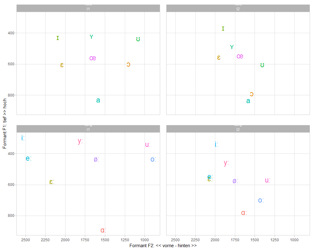

webshot("tmp.html","pictures/vokalformanten_interaktiv_l1_l2_lang_kurz.pdf", delay =5, vwidth = 800, vheight=600)

9.4.1.4 Diagramm 2 (statisch)

vgl_pivot <- vergleich %>% 
  group_by(vokal) %>% 
  pivot_longer(f1_l1:dauer_l2, names_to = "category", values_to = "value") %>% 
  separate(category, into = c("category", "l1_l2")) %>% 
  drop_na() %>% 
  pivot_wider(names_from = category, values_from = value)
vgl_pivot %>% rmarkdown::paged_table()

(graph2 <- vgl_pivot %>% 
  drop_na() %>% 
  group_by(vowel_ipa, l1_l2, lange) %>% 
  ggplot(aes(f2,f1)) +
  geom_hex(alpha = 0.2, show.legend = F) +
  geom_text(aes(label = vowel_ipa, color = vowel_ipa), 
            vjust = 1, hjust = 1, check_overlap = T, show.legend = F, size = 6) +
  scale_y_reverse() +
  scale_x_reverse(breaks = c(1000, 1250, 1500, 1750, 2000, 2250, 2500)) +
  facet_wrap(~ l1_l2) +
  theme_light() + 
  labs(y = "Formant F1: tief >> hoch",
       x = "Formant F2: << vorne - hinten >>")
)

ggsave("pictures/vergleich_vokalformanten_lang_kurz_ipa.jpg")

9.4.1.5 Diagramm 2 (interaktiv)

library(plotly)
ggplotly(graph2) %>% layout(showlegend = FALSE)

9.4.1.6 Diagramm 5 (statisch)

vgl_pivot <- vergleich %>% 
  group_by(vowel_ipa) %>% 
  pivot_longer(f1_l1:dauer_l2, names_to = "category", values_to = "value") %>% 
  separate(category, into = c("category", "l1_l2")) %>% 
  drop_na() %>% 
  pivot_wider(names_from = category, values_from = value)
vgl_pivot %>% rmarkdown::paged_table()

(graph5 <- vgl_pivot %>% 
  drop_na() %>% 
  group_by(vowel_ipa, l1_l2) %>% 
  ggplot(aes(f2,f1)) +
  geom_hex(alpha = 0.2, show.legend = F) +
  geom_text(aes(label = vowel_ipa, color = vowel_ipa), 
            size = 6, vjust = 1, hjust = 1, check_overlap = T, show.legend = F) +
  scale_y_reverse() +
  scale_x_reverse(breaks = c(1000, 1250, 1500, 1750, 2000, 2250, 2500)) +
  facet_wrap(~ l1_l2) +
  theme_light() + 
  labs(y = "Formant F1: tief >> hoch",
       x = "Formant F2: << vorne - hinten >>")
)

ggsave("pictures/vergleich_vokalformanten.jpg")

9.4.1.7 Diagramm 5 (interaktiv)

library(plotly)
ggplotly(graph5) %>% layout(showlegend = FALSE)

9.4.1.8 Diagramm 6 (statisch)

vgl_pivot <- vergleich %>% 
  group_by(vowel_ipa) %>% 
  pivot_longer(f1_l1:dauer_l2, names_to = "category", values_to = "value") %>% 
  separate(category, into = c("category", "l1_l2")) %>% 
  drop_na() %>% 
  pivot_wider(names_from = category, values_from = value)
vgl_pivot %>% rmarkdown::paged_table()

(graph6 <- vgl_pivot %>% 
  drop_na() %>% 
  group_by(vowel_ipa, l1_l2, lange) %>% 
  ggplot(aes(f2,f1)) +
  geom_hex(alpha = 0.2, show.legend = F) +
  geom_text(aes(label = vowel_ipa, color = vowel_ipa), 
            size = 6, vjust = 1, hjust = 1, check_overlap = T, show.legend = F) +
  scale_y_reverse() +
  scale_x_reverse(breaks = c(1000, 1250, 1500, 1750, 2000, 2250, 2500)) +
  facet_wrap(~ lange + l1_l2) +
  theme_light() + 
  labs(y = "Formant F1: tief >> hoch",
       x = "Formant F2: << vorne - hinten >>")
)

ggsave("pictures/vergleich_vokalformanten_lang_kurz.jpg")

9.4.1.9 Diagramm 6 (interaktiv)

library(plotly)
ggplotly(graph6) %>% layout(showlegend = FALSE)

9.4.2 Datensatz 3

9.4.2.1 Diagramm 3a alle Vokale (statisch)

Messungen von TP mit Praat-Script (👉 Matt Winn: https://github.com/mwinn83)

library(ggrepel)

(graph3a <- df %>% 
   filter(speaker != "Monika1") %>% 
    group_by(vowel, speaker, vowel_ipa) %>% 
  summarise(f1 = mean(F1),
            f2 = mean(F2)) %>% 
  ggplot(aes(f2,f1)) +
  geom_hex(alpha = 0.2, show.legend = F) +
  geom_text(aes(label = vowel_ipa, color = vowel_ipa),
            vjust = 1, hjust = 1, check_overlap = T, show.legend = F, size = 5) +
  # geom_label_repel(aes(label = IPA, color = IPA),
  #           vjust = 1, hjust = 1, check_overlap = T, show.legend = F, size = 5) +
  scale_y_reverse() +
  scale_x_reverse(breaks = c(1000, 1250, 1500, 1750, 2000, 2250, 2500)) +
  facet_wrap(~ speaker) +
  # theme_light() + 
  theme(axis.text.x = element_text(angle = 60, hjust = 1)) +
  labs(y = "Formant F1: tief >> hoch",
       x = "Formant F2: << vorne - hinten >>")
 )

ggsave("pictures/messungen_tp_vokalformanten_ipa.jpg", dpi = 100, width = 10, height = 10)

9.4.2.2 Diagramm 3a alle Vokale (interaktiv)

library(plotly)
ggplotly(graph3a) %>% layout(showlegend = FALSE)

9.4.2.3 Diagramm 3b kurze Vokale (statisch)

library(ggrepel)

(graph3b <- df %>% 
    mutate(lange = ifelse(
      vowel %in% c("I","E","Y","OE","a","O","U"), "kurz","lang")) %>% 
   filter(speaker != "Monika1") %>% 
    filter(lange == "kurz") %>% 
    group_by(vowel, speaker, vowel_ipa) %>% 
  summarise(f1 = mean(F1),
            f2 = mean(F2)) %>% 
  ggplot(aes(f2,f1)) +
  geom_hex(alpha = 0.2, show.legend = F) +
  geom_text(aes(label = vowel_ipa, color = vowel_ipa),
            vjust = 1, hjust = 1, check_overlap = T, show.legend = F, size = 5) +
  # geom_label_repel(aes(label = IPA, color = IPA),
  #           vjust = 1, hjust = 1, check_overlap = T, show.legend = F, size = 5) +
  scale_y_reverse() +
  scale_x_reverse(breaks = c(1000, 1250, 1500, 1750, 2000, 2250, 2500)) +
  facet_wrap(~ speaker) +
  # theme_light() + 
  theme(axis.text.x = element_text(angle = 60, hjust = 1)) +
  labs(y = "Formant F1: tief >> hoch",
       x = "Formant F2: << vorne - hinten >>")
 )

ggsave("pictures/messungen_tp_vokalformanten_ipa_kurz.jpg", dpi = 100, width = 10, height = 10)

9.4.2.4 Diagramm 3b kurze Vokale (interaktiv)

library(plotly)
ggplotly(graph3b) %>% layout(showlegend = FALSE)

9.4.2.5 Diagramm 3c lange Vokale (statisch)

library(ggrepel)

(graph3c <- df %>% 
    mutate(lange = ifelse(
      vowel %in% c("I","E","Y","OE","a","O","U"), "kurz","lang")) %>% 
   filter(speaker != "Monika1") %>% 
    filter(lange == "lang") %>% 
    group_by(vowel, speaker, vowel_ipa) %>% 
  summarise(f1 = mean(F1),
            f2 = mean(F2)) %>% 
  ggplot(aes(f2,f1)) +
  geom_hex(alpha = 0.2, show.legend = F) +
  geom_text(aes(label = vowel_ipa, color = vowel_ipa),
            vjust = 1, hjust = 1, check_overlap = T, show.legend = F, size = 5) +
  # geom_label_repel(aes(label = IPA, color = IPA),
  #           vjust = 1, hjust = 1, check_overlap = T, show.legend = F, size = 5) +
  scale_y_reverse() +
  scale_x_reverse(breaks = c(1000, 1250, 1500, 1750, 2000, 2250, 2500)) +
  facet_wrap(~ speaker) +
  # theme_light() + 
  theme(axis.text.x = element_text(angle = 60, hjust = 1)) +
  labs(y = "Formant F1: tief >> hoch",
       x = "Formant F2: << vorne - hinten >>")
 )

ggsave("pictures/messungen_tp_vokalformanten_ipa_lang.jpg", dpi = 100, width = 10, height = 10)

9.4.2.6 Diagramm 3c lange Vokale (interaktiv)

library(plotly)
ggplotly(graph3c) %>% layout(showlegend = FALSE)

9.5 Aggregierter Datensatz

Grundlage ist Datensatz 1

9.5.1 IPA syms

ipa_vow2 <- c(
a = "\u0061",
AA = "\u0251\u02D0",
E = "\u025B",
ee = "\u0065\u02D0",
EE = "\u025B\u02D0",
I = "\u026A",
ii = "\u0069\u02D0",
O = "\u0254",
OE = "\u0153",
oo = "\u006F\u02D0",
oe = "\u00F8\u02D0",
U = "\u028A",
Y = "\u028F",
uu = "\u0075\u02D0",
yy = "\u0079\u02D0"
)

ipavow2 = ipa_vow2 %>%  as_tibble() %>% rename(vowel = value)

9.5.2 Tabelle

Mittelwerte aus Datensatz 1

vokale_agg <- vokale %>% 
  group_by(vokal, lange, l1_l2) %>% 
  summarise(f1_avg = mean(f1),
            f2_avg = mean(f2),
            dauer_avg = mean(dauer))

vokale_agg1 <- vokale_agg %>% filter(l1_l2 == "L1") %>% cbind(ipavow2)
vokale_agg2 <- vokale_agg %>% filter(l1_l2 == "L2") %>% cbind(ipavow2)
vokale_agg <- rbind(vokale_agg1, vokale_agg2) %>% as_tibble()

vokale_agg %>% rmarkdown::paged_table()

9.5.3 Datensatz 1 mit aggregierten Daten

9.5.3.1 Diagramm 4 (statisch)

library(tidytext)
library(ggrepel)

(graph4 <- vokale %>% 
  group_by(vokal, l1_l2, color = vowel_ipa, label = vowel_ipa, fill = vowel_ipa, shape = vowel_ipa) %>% 
  ggplot(aes(f2,f1)) +
  geom_hex(alpha = 0.2, show.legend = F) +
  geom_label(data = vokale_agg, label = vokale_agg$vowel, aes(x = f2_avg, y = f1_avg), color = "black") + 
  stat_ellipse(level = 0.67, geom = "polygon", alpha = 0.2) +
  scale_color_discrete(breaks = c("a","a:","e:","E","E:","I","i:","O","o:","U","u:","Y","y:","Ö","ö")) +
  # geom_text(aes(label = vokal, color = vokal), vjust = 1, hjust = 1, check_overlap = T, show.legend = F) +
  scale_y_reverse() +
  scale_x_reverse() +
  facet_wrap(~ l1_l2) +
  theme_light() + 
  guides(color = FALSE) +
  labs(y = "Formant F1: tief >> hoch",
       x = "Formant F2: << vorne - hinten >>")
)

9.5.3.2 Diagramm 7 (statisch)

(graph7 <- vokale_agg %>% 
  group_by(vokal, l1_l2, label = vowel) %>% 
  ggplot(aes(f2_avg,f1_avg)) +
  geom_hex(alpha = 0.2, show.legend = F) +
  geom_text(aes(label = vowel, color = vowel), 
            size = 6, vjust = 1, hjust = 1, check_overlap = T, show.legend = F) +
  scale_y_reverse() +
  scale_x_reverse() +
  facet_wrap(~ l1_l2) +
  theme_light() + 
  labs(y = "Formant F1: tief >> hoch",
       x = "Formant F2: << vorne - hinten >>")
)

ggsave("pictures/vokalformanten.jpg")

9.5.3.3 Diagramm 5 (interaktiv)

Interaktives Diagramm mit dem plotly-Programm:

library(plotly)
ggplotly(graph7) %>% layout(showlegend = FALSE)

9.6 Abbildungen mit phonR

Abbildungen mit dem phonR-Paket, spezialisiert auf die graphische Darstellung von akustischen, insbesondere phonetischen Daten.

9.6.0.1 Diagramm 8

Aggregierter Datensatz

library(phonR)

par(mfrow = c(1, 1))
with(vokale_agg, plotVowels(f1_avg, f2_avg, vowel, group = lange, pch.tokens = vowel, cex.tokens = 1.2, 
    alpha.tokens = 0.3, plot.means = TRUE, pch.means = vowel, cex.means = 2, var.col.by = vowel, 
    var.sty.by = lange, hull.fill = TRUE, hull.line = TRUE, fill.opacity = 0.1, 
    pretty = TRUE))

# Bild auf Festplatte speichern in drei Schritten:
# 1. Open jpeg file
jpeg("pictures/phonR_vowel_space.jpg", 
     width = 840, height = 535)

# 2. Create the plot
par(mfrow = c(1, 1))
with(vokale_agg, plotVowels(f1_avg, f2_avg, vowel, group = lange, pch.tokens = vowel, cex.tokens = 1.2, 
    alpha.tokens = 0.3, plot.means = TRUE, pch.means = vowel, cex.means = 2, var.col.by = vowel, 
    var.sty.by = lange, hull.fill = TRUE, hull.line = TRUE, fill.opacity = 0.1, 
    pretty = TRUE))

# 3. Close the file
dev.off()

## cairo_pdf 
##         2

9.6.0.2 Diagramm 9

Einzelne Messungen

library(phonR)

par(mfrow = c(1, 1))
with(vokale, plotVowels(f1, f2, vowel_ipa, group = lange, pch.tokens = vowel_ipa, cex.tokens = 1.2, 
    alpha.tokens = 0.3, plot.means = TRUE, pch.means = vowel_ipa, cex.means = 2, var.col.by = lange, 
    var.sty.by = lange, hull.fill = TRUE, hull.line = TRUE, fill.opacity = 0.1, 
    pretty = TRUE))

# Bild auf Festplatte speichern in drei Schritten:
# 1. Open jpeg file
jpeg("pictures/phonR_vowel_space2.jpg", 
     width = 840, height = 535)

# 2. Create the plot
par(mfrow = c(1, 1))
with(vokale, plotVowels(f1, f2, vowel_ipa, group = lange, pch.tokens = vowel_ipa, cex.tokens = 1.2, 
    alpha.tokens = 0.3, plot.means = TRUE, pch.means = vowel_ipa, cex.means = 2, var.col.by = lange, 
    var.sty.by = lange, hull.fill = TRUE, hull.line = TRUE, fill.opacity = 0.1, 
    pretty = TRUE))

# 3. Close the file
dev.off()

## cairo_pdf 
##         2